Lab 7: Kalman Filter

Task 1: Estimate Drag and Momentum

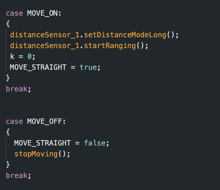
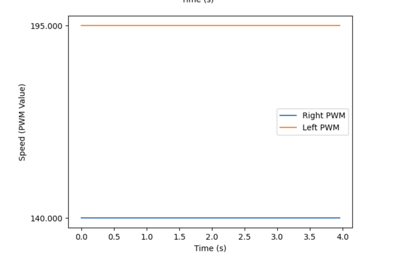
In order to generate data to calculate drag and momentum, I used a step response. I drove the robot to the wall at a constant PWM value of 195, which was similar to the PWM values used in Lab 5. To code the step response and record distance data, I made cases MOVE_ON and MOVE_OFF to turn the flag MOVE_STRAIGHT on and off.

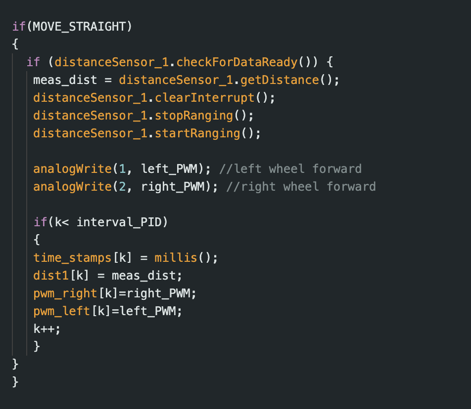
When MOVE_STRAIGHT was activated, the following portion of the loop function would execute. This allowed the robot to move forward while also recording time, distance, and motor input data.

Once the code was set up, I gathered the step response data. The video below shows the trial during which I collected the data used for tasks 1, 2, and 3.

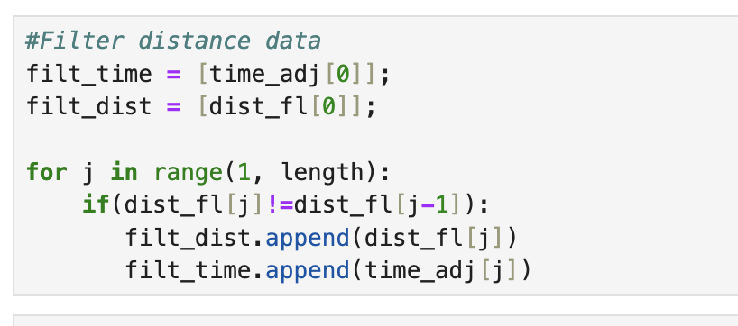
Before I could calculate velocity from the distance and time values, I first had to filter the data. I did this by checking whether a distance measurement was equivalent to the previous one. If it was different, it could be added to the distance array that would be used to calculate velocity. This prevented me from accidentally calculating velocity values of zero.

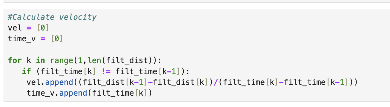
Once the distance data was filtered, I calculated velocity as shown in the code below.

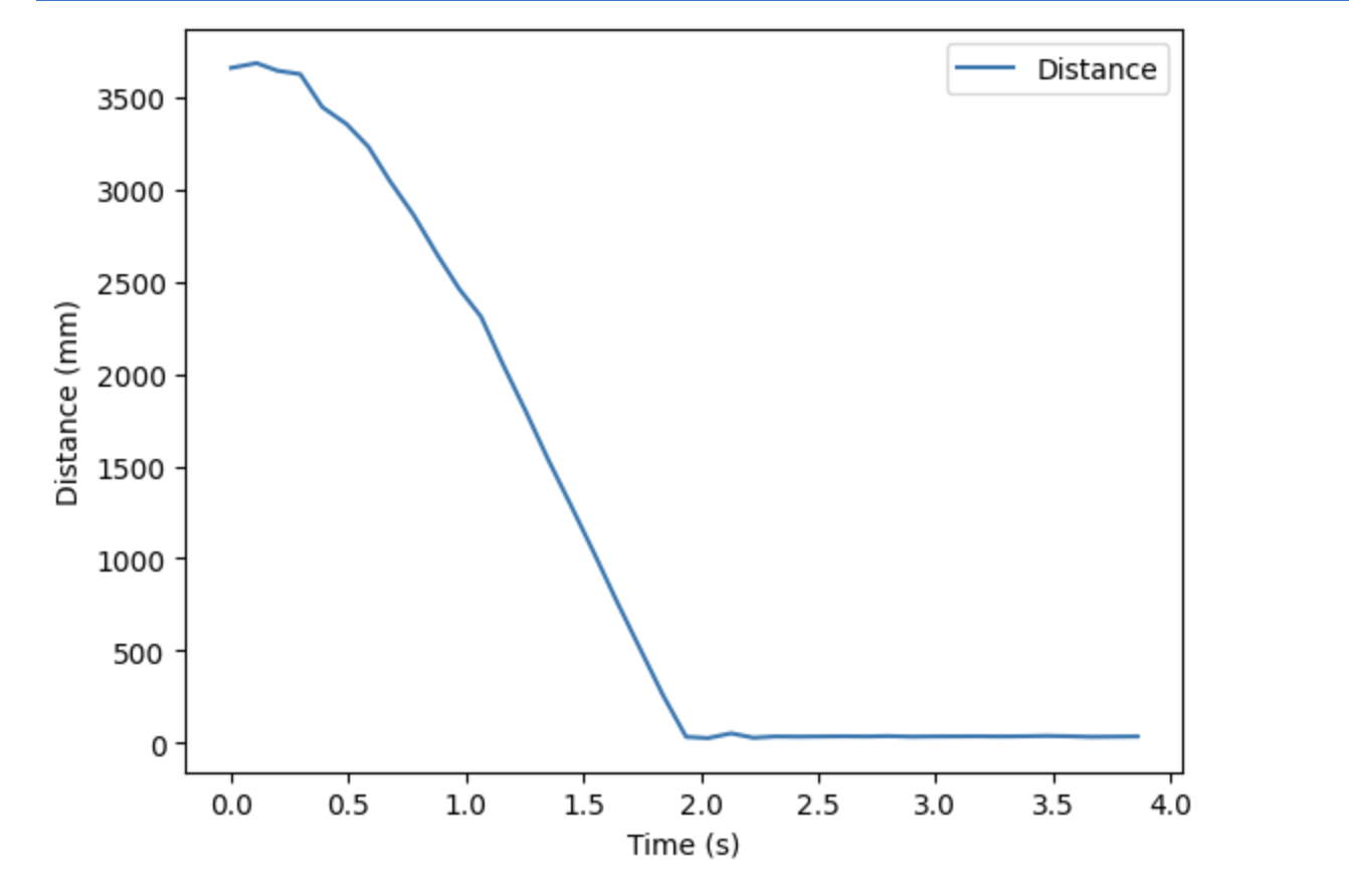
After I obtained velocity, I was able to plot distance, velocity, and motor input over time. The slope of the distance plot steadily increases until about 1 second, when it stabilizes. This behavior approximately matches the velocity plot, which reaches its steady state value shortly after 1 second.

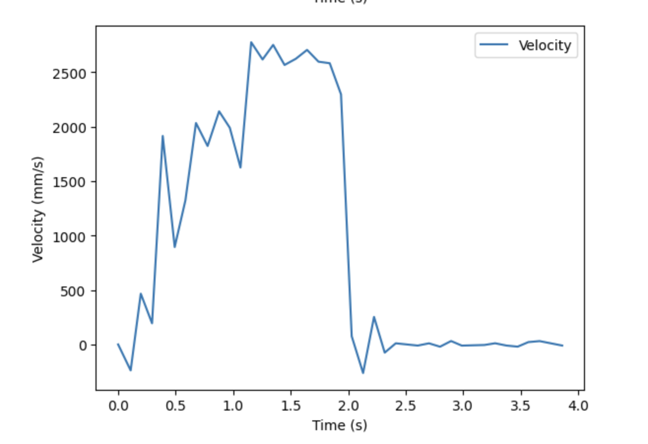
Using the velocity data, I found the steady state velocity to be approximately 2661 mm/s. 90% of the steady state velocity would be 2395 mm/s. However, none of the data points collected matched this value. But, a velocity of 2140 mm/s was calculated at 0.878 seconds. This velocity is 80% of the steady state, so I was able to use 0.878 as the 80% rise time. This is the value I used to calculate m, as seen below.

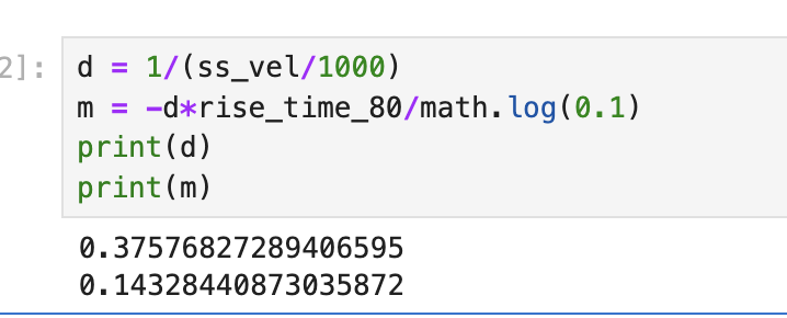
Based on my data, I found the mass to be 0.143 kg, and the drag to be 0.376 kg/s.

Task 2: Initialize KF

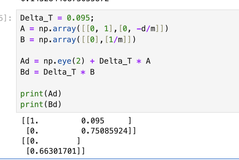
Using the drag and mass calculations above, I was able to find the A and B matrices. To determine dt, I found that the TOF sensor took about 10.5 samples per second, or 1 sample every 95 ms. Using A, B, and dt, I was able to calculate Ad and Bd, as shown below.

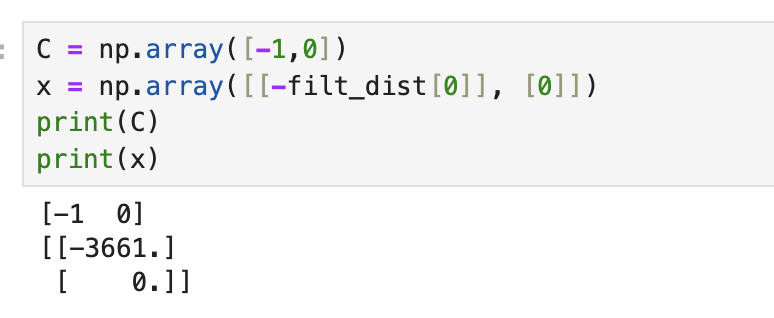
I then defined C and x as shown below.

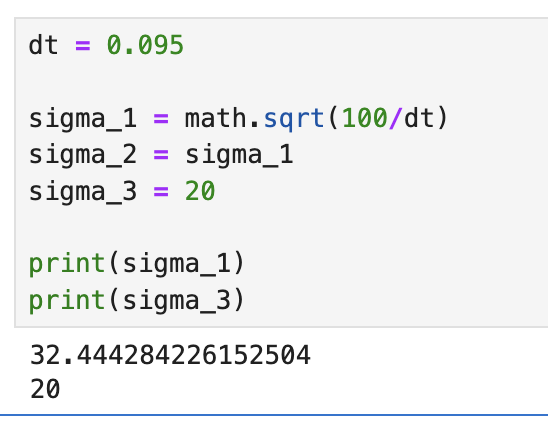
Next, I calculated the covariances sigma_1, sigma_2, which depended on dt. I set sigma_3 to 20, based on the values found in the TOF sensor datasheet. Sigma_3 represents the variation in the TOF sensor readings, and according to the data sheet long distance mode has a ranging error of +/- 20 mm.

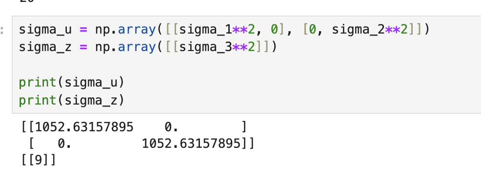
Using these covariance values, I was able to specify the covariance matrices, as shown below.

Task 3: Implement and Test Kalman Filter in Jupyter

Using the code given in the lab instructions, I was able to implement the Kalman filter in Jupyter. First, though, I had to initialize my intial state, x, and the covariance matrix, sigma. I started with covariance values of 4 and 4, as seen in the code below. The new distance values outputted by the function given were stored in the kf_output array.

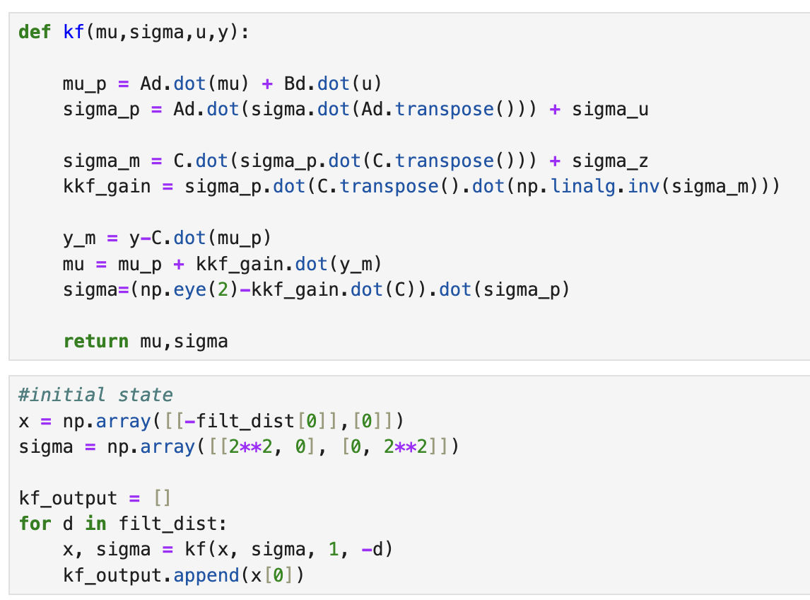
Once I obtained the filtered distance values, I plotted against the original distance values, as shown below.

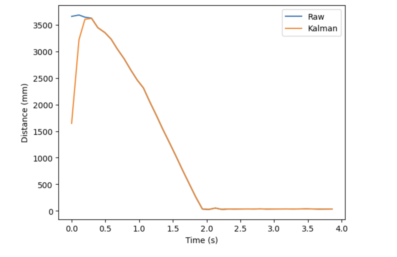
Even with covariance values as low as 4, the filtered distance values were pretty similar to my initial recorded distances. Increasing the covariance does not change the plot significantly, since the Kalman data already overlaps the raw data starting at 0.5 seconds. However, there is some strange behavior at the beginning of the plot. This “tail” does not seem to shrink even as I change the covariance matrix. However, I found that decreasing the value of sigma_3 was able to reduce this discrepancy between the filtered and raw data. The resulting plot for sigma_3 = 2 is shown below.

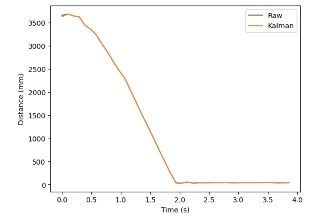
In this case, decreasing, not increasing, a covariance value gave me better results. This suggests that I was greatly overestimating the variance in my TOF sensor readings, at least for this trial, since it gave me very consistent readings.

Task 4: Implement the Kalman Filter on the Robot

I did not have time to do this task. When I initially read the lab, I assumed, although incorrectly, that this part was optional. I was not aware that we were supposed to do it until I saw the Ed post made by Professor Helbling after my class that ended at 9 pm today. Unfortunately, that warning did not come early enough for me to work on this portion of the lab.

I will hopefully complete this task in conjunction with Lab 8 so that I can get better results with my stunt. So, check back later for more progress on this portion of the lab :)

Acknowledgements:

I referred to Stefan’s lab 7 from last year to see a more in-depth explanation on how to calculate drag and mass from the values obtained from the step-input. In addition, I found Mikayla’s explanation of how to find the covariances very informative.

referred to Stefan for how to calculate drag & mass referred to Mikayla for how to find covariances