Lab 3

Prelab

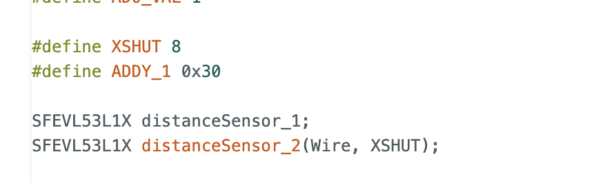
Throughout this lab, we worked with Time-of-Flight (ToF) distance sensors. According to the corresponding datasheet, the default I2C address for a ToF sensor is 0x52. Since we will be using two sensors during the lab, one of the addresses will need to be changed in order to get distance readings from both at the same time. This will be done by wiring pin 8 on the Artemis board to the XSHUT pin on one sensor. This configuration is shown on the wiring diagram below. In addition to the XSHUT pin, the wiring diagram shows how the other ToF pins will be connected to the QWIIC connector.

Since the ToF sensors will be essential for regulating the robot’s movement, they should be attached to the longer QWIIC connectors. This increases the flexibility of their positioning, allowing them to be placed on the front, sides, or back as necessary. For example, it would be beneficial to have one sensor on the front and one on the right side of the car if I am navigating following the wall to my right. But, if I just want to prevent crashes it might be better to have one on the back instead of the front of the car.

Task 1: Connect Components

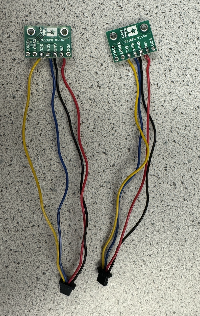
During lab, the ToF sensors were soldered to the longer QWIIC connectors in accordance with the wiring diagram shown above. This is shown in the images below.

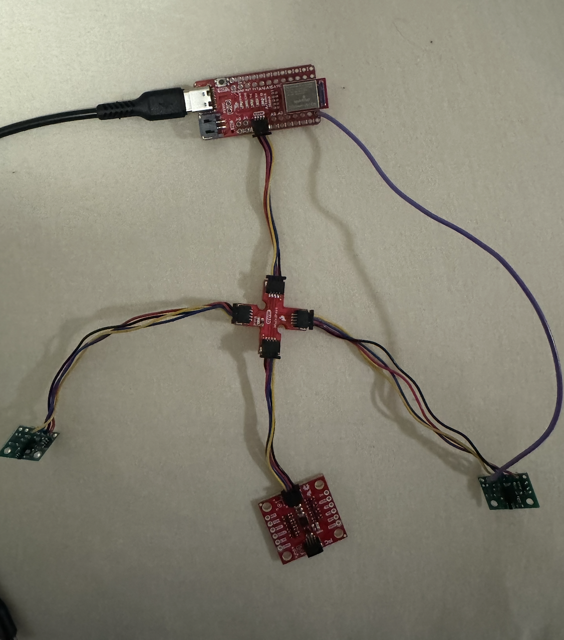
Next, the QWIIC connectors were connected to the QWIIC breakout board. The IMU was also attached to the breakout board via a shorter QWIIC connector. Then, the QWIIC breakout board was connected to the Artemis board. In addition, the battery was soldered to JST jumper wires in order for it to connect to the Artemis board. The full configuration, minus the battery, is shown below.

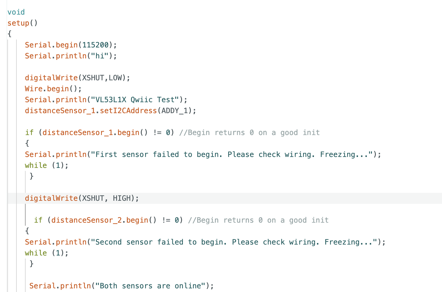
Task 2: Scan for I2C Device

Running Example1_wire_I2C gave 0x29 as the I2C address for the ToF sensor. This output is shown below.

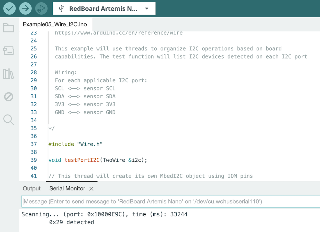
As mentioned in the prelab, the expected I2C address is 0x52. This occurs because the binary form of 0x52 gets shifted 1 place to the right, resulting in 0x29.

Task 3: Choose ToF Mode

The short mode is likely ideal for the final robot. The car is quite small, so a maximum distance of 1.3 meters should suffice in preventing the robot from going too far off course. In addition, the short mode is least sensitive to ambient light, which is likely to be present in most settings where the robot is used. The maximum distance measured by long mode actually decreases to less than the short mode’s maximum when it’s placed in ambient light. As a resut, accuracy will be higher in the short mode, making it the better choice.

Task 4: Test ToF Short Mode

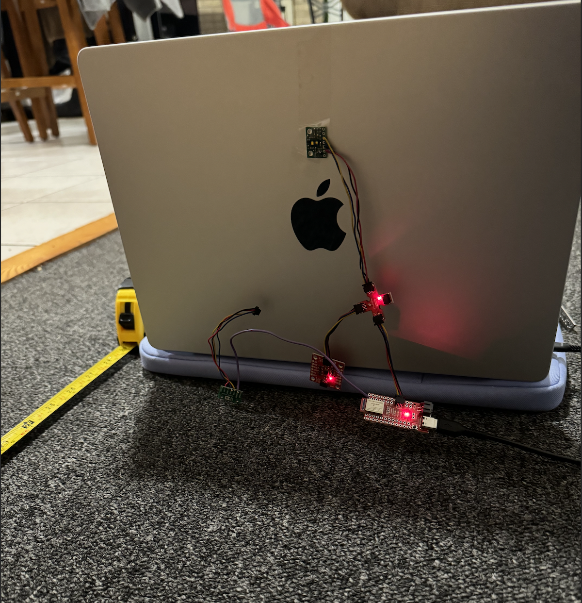
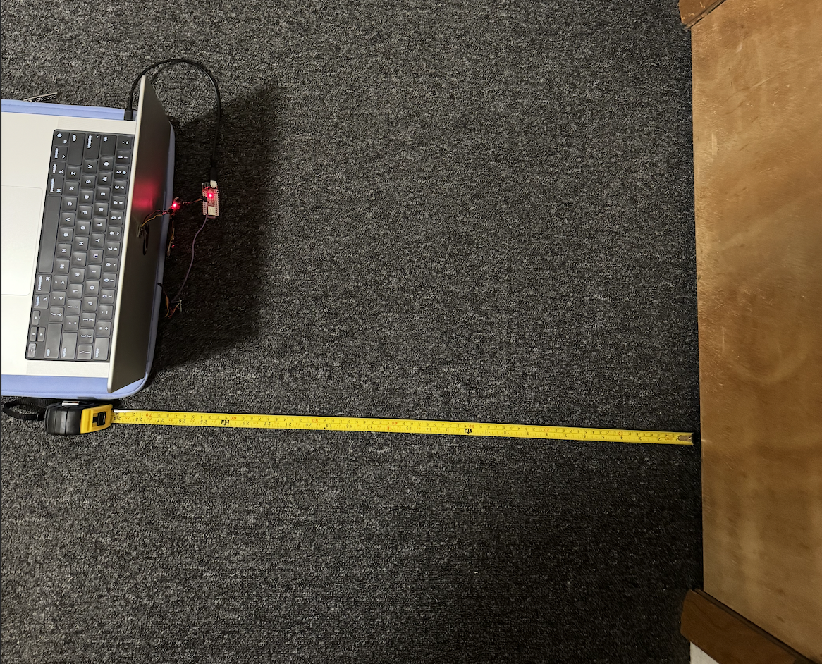
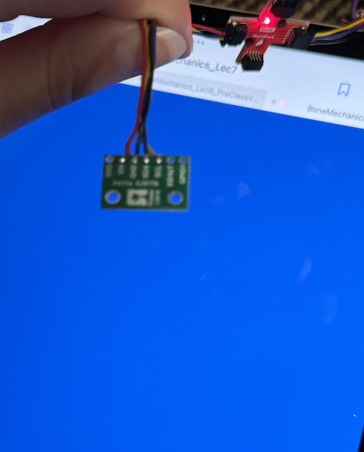
In order to test the short mode of my ToF sensor, I taped the sensor to the back of my laptop and lined it up parallel to a wall. The setup is shown in the images below.

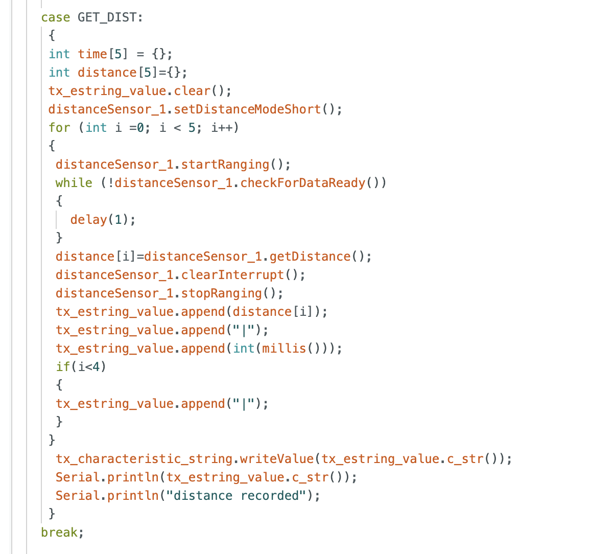
I took measurements at distances ranging from 5 to 130 cm. At each distance measured, I collected 5 data points from the sensor in order to obtain repeatability data. The Arduino code written for this task is shown below.

The data was then processed in Python at each distance. An example of how this was done for the 10 cm distance is shown below.

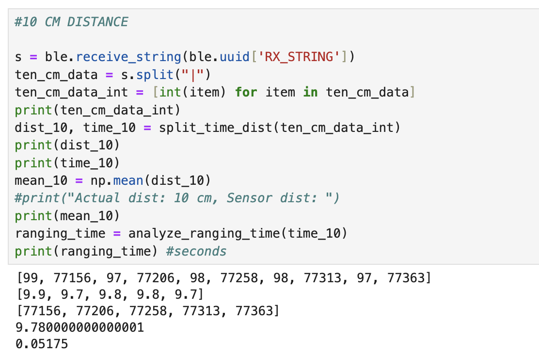
As seen in the code, part of the data processing included calculating the mean at each distance. This allowed the mean of the measured data be plotted against the actual distance. This graph is shown below.

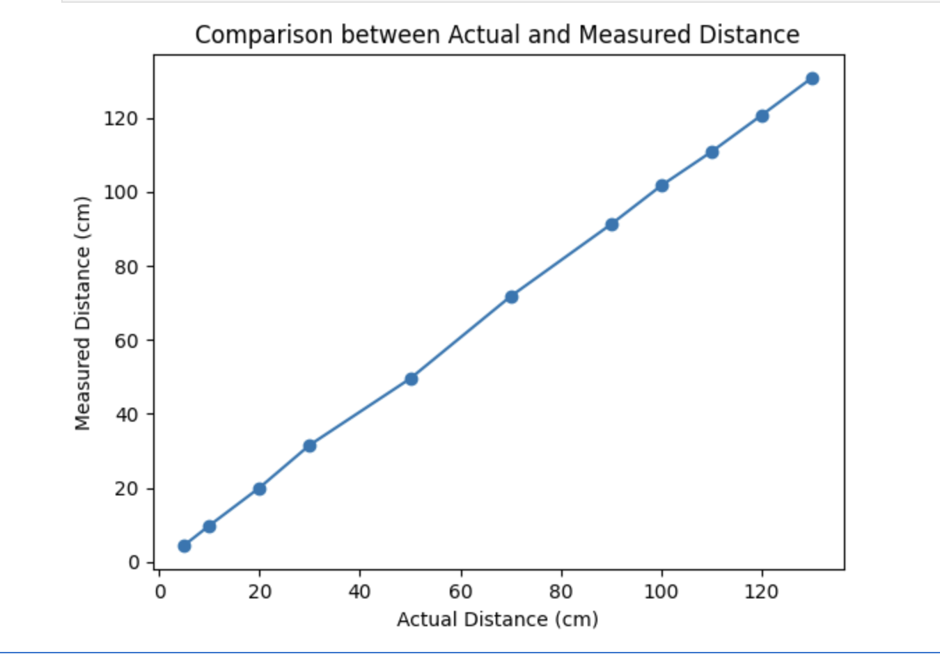
As seen above, there was a linear relationship between the actual and measured distances over the whole range of distances. To examine the accuracy results more closely, I also plotted the difference between the measured and actual distances over the distance range.

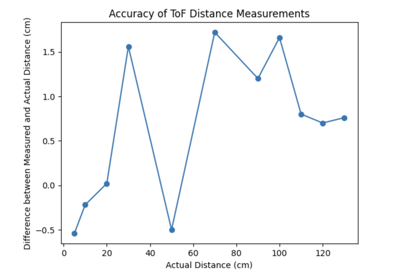
As shown in the plot above, the measured distance values were pretty accurate throughout the range, deviating about 1.5 cm at most. It does seem that accuracy decreases slightly as distance increases, but the difference is still quite small compared to the order of magnitude of the measured value. For example, at a distance of 100 cm, there is an approximately 1.5 cm deviation. However, this is only a 1.5% error, demonstrating that the distance values are quite accurate.

The standard deviation was calculated at each distance value to determine repeatability. The plot of standard deviation over distance is shown below.

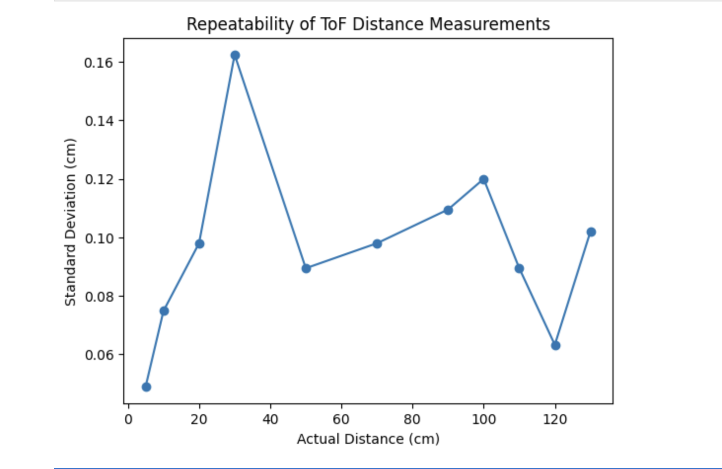
As shown in the plot, the standard deviation between data points is very small. This shows that the ToF distance values should be repeatable. However, it is important to note that these values were taken while the sensors were stationary, which will not be the case once they are affixed to the robot.

Finally, I calculated the ranging time at each distance, which is the time between each data point collected by the ToF sensor. The code I used to calculate it in Python is displayed below.

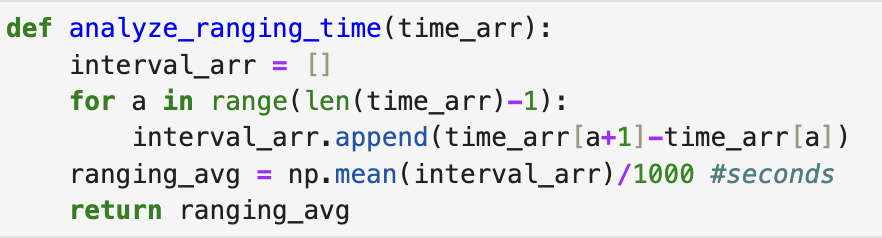
The ranging time remained relatively the same, even as distance increased. It ranged between 0.0505 and 0.05275 seconds.

Task 5: Sensors in Parallel

As discussed in the prelab, using both sensors in parallel requires changing the address of one of the sensors. In addition to doing this manually with wiring, the new address needs to be specified in the Arduino code. The code I used to do this is shown below.

The setup had to be changed as well. To ensure the first sensor is set to the new address, the XSHUT pin must be set to low. Then, once the first sensor is running, the XSHUT pin can be set back to high. The Arduino code for this can be seen below.

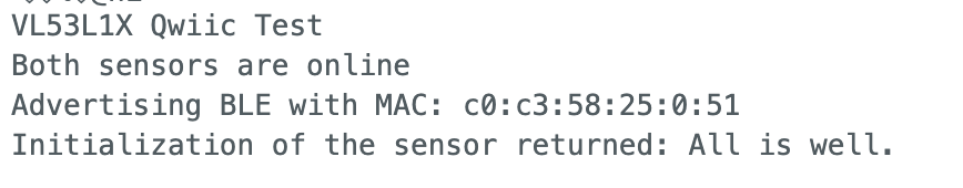
The Serial output displayed below shows that both sensors were able to connect properly once these changes were made.

Task 6:

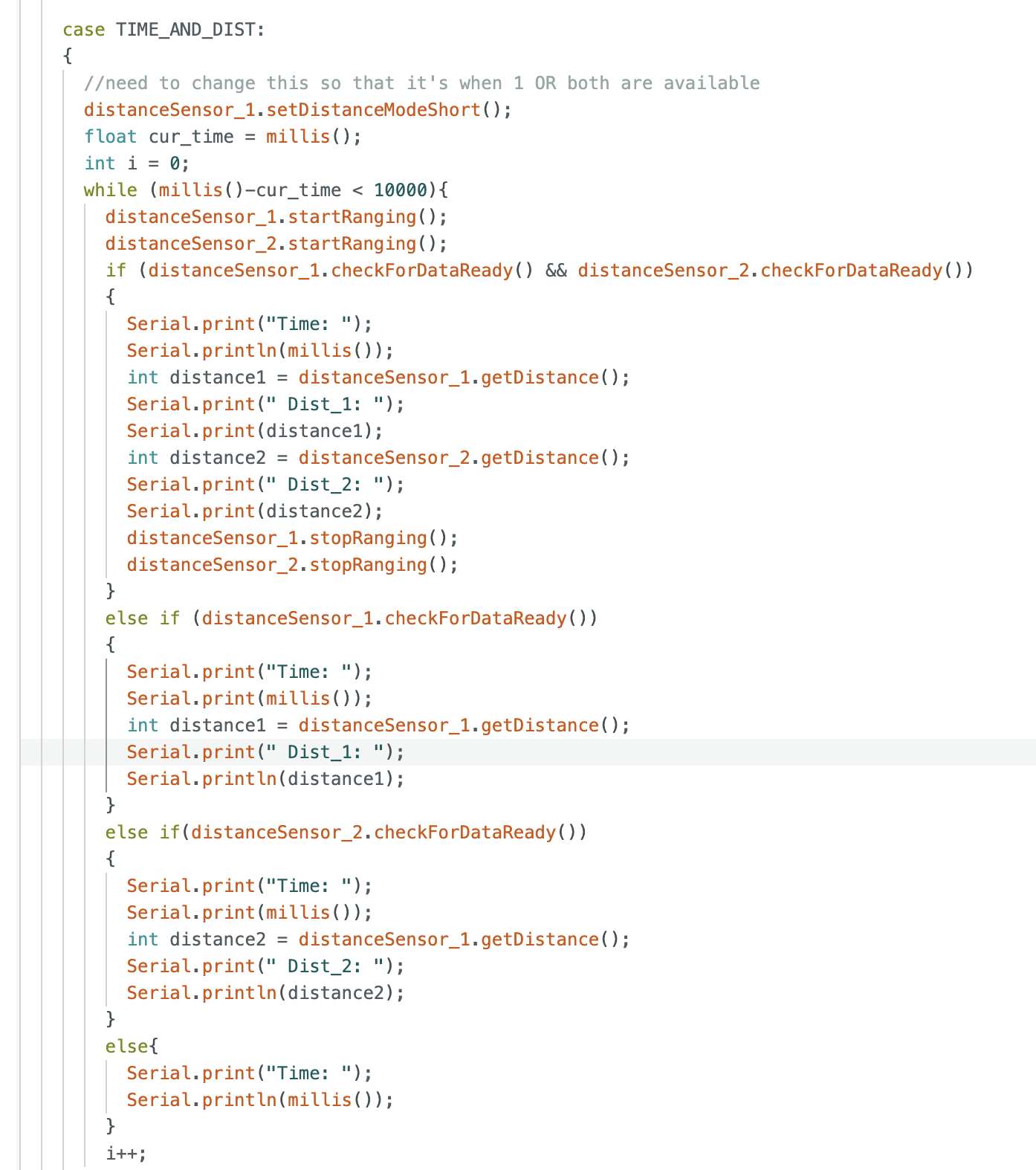
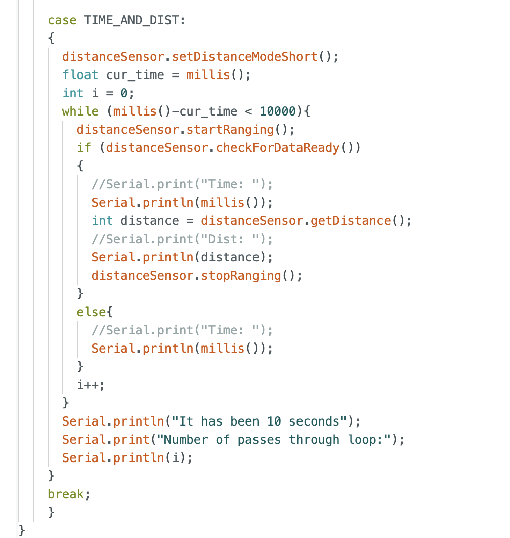
The ToF sensors take a bit of time to update with new measurements. In order to prevent this from causing delays in robot response time, I wrote the following code, which prints time continuously, adding in distance measurements from either or both sensors when they are ready.

The following embedded video shows this code in action.

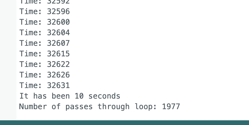
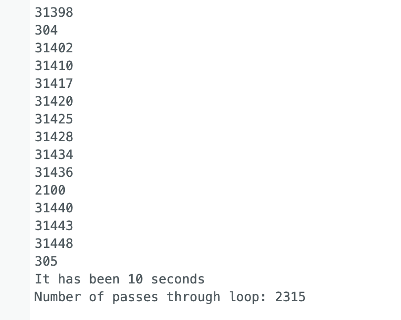
With comments labeling the data output, the loop executes 1977 times in 10 seconds, or at a rate of 199.7 times/second. Removing these comments increases the rate to 231.5 times/second. Screenshots of the Serial monitor output that corresponds to these two cases is shown below.

I also tested just one sensor. This led to much faster rates of 368.2 times/second with comments and 499.9 times/second without. The code and resulting Serial monitor screenshots are shown below.

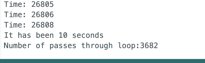
This code required fewer calls of checkforDataReady() and startRanging() since there was only one sensor instead of two. This indicates that these commands are limiting factors that prevent the loop from executing any faster.

Task 7:

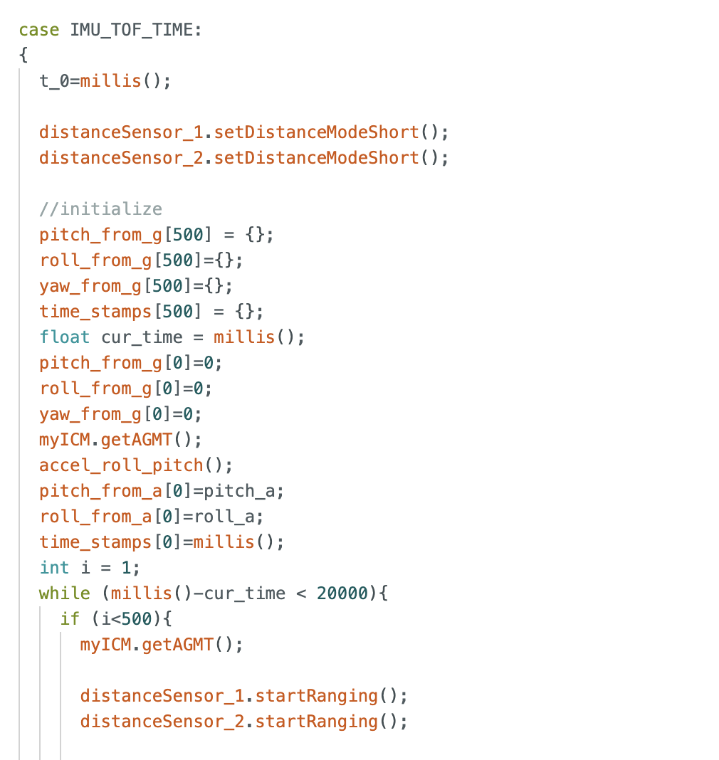
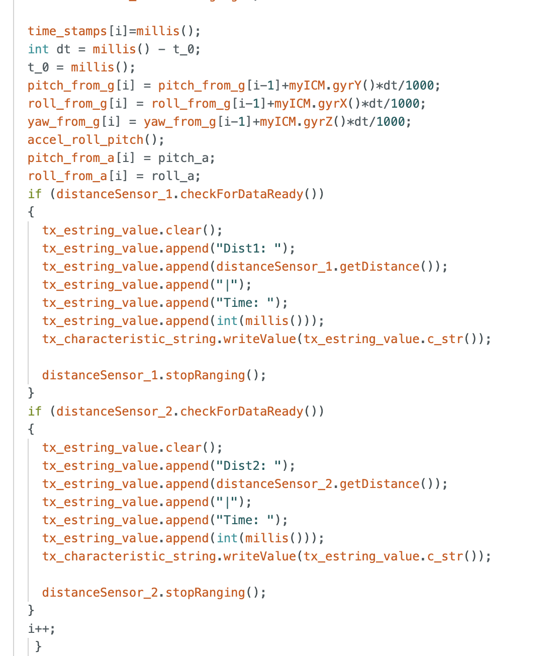
The final step in this lab was to integrate the ToF sensors with the IMU. Since the IMU and the ToF sensors do not have measurements available at the same intervals, I had to make the time stamps recorded for each sensor were unique. I did this by writing a command in Arduino that looped through collecting IMU values, and outputting distance values when they are available. The code for this loop is displayed below.

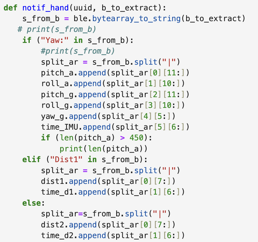
The data collected from the IMU and ToF was receieved and handled by my new notification handler. This Python code is shown below.

After the data was processed by the notification handler, I plotted both IMU and the ToF data over time. Both plots are shown below.

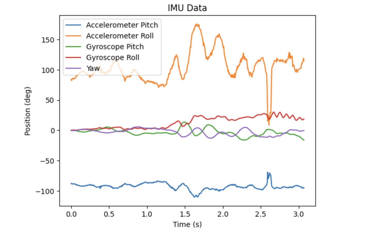
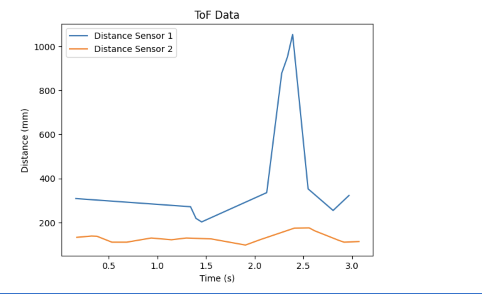
When the data shown in these plots was collected, the ToF were being held mostly steady, but the IMU sensor was oscillating slightly. However, at around 2.4 seconds Sensor 1 was moved a bit abrupty, causing a rapid change in distance recorded. In reality, it did not move quite that far, but it likely lost sight of the original reference point since it was twisted in the air, leading to the rapid change in measured distance. Interestingly, it is evident that this abrupt change corresponded with a change in roll, as recorded by the accelerometer data seen on the IMU plot.

5000 Level Tasks

Task 1: Discussion on Infrared Transmission Based Sensors

Two types of infrared sensors are Time-of-Flight (ToF) sensors, which were used in this lab, and Reflective Infrared (IR) Sensors. ToF sensors work by measuring the amount of time it takes for light to an obstacle and back. They send light in pulses and are able to calculate the distance by multiplying time by the speed of light.

Reflective IR sensors work via triangulation. They emit light from one side and detect the angle of the reflected light from the other. Based on this angle, the distance to the obstacle can be calculated.

Reflective IR sensors work very well at short distances, so they are great for detection applications. In addition, they are cheaper than ToF sensors. But, ToF sensors are able to work more accurately over a larger range of distances, as shown in this lab.

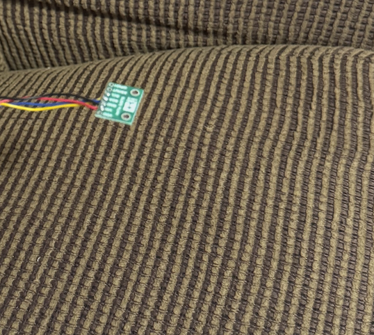
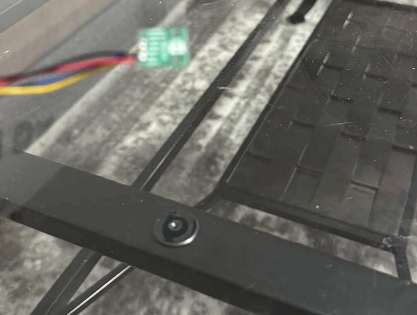
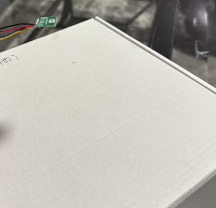
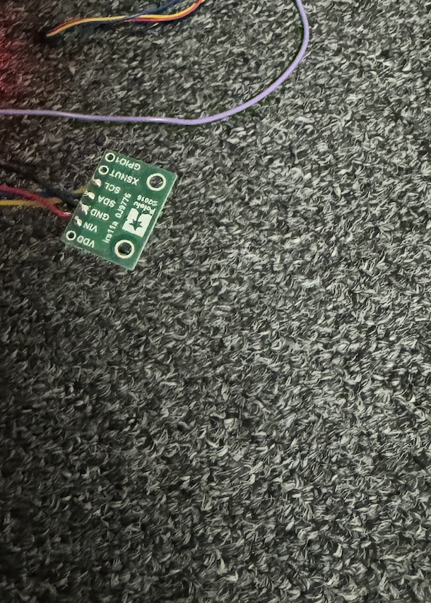
Task 2: ToF Sensitivity to Colors and Textures

I tested the ToF sensor on four different textures: felt (couch), glass, cardboard, and carpet. Pictures of these textures are shown below.

The sensor was placed 15 cm from the textured object, and 5 distance measurements were taken. The average distance output for each item is shown below.

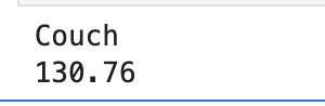
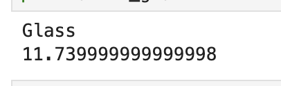
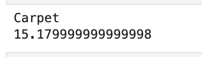
As seen in the images, the cardboard and carpet gave pretty accurate measurements. However, the glass appeared closer than it actually was, and the sensor had significantly more trouble getting an accurate reading for the couch (felt). These discrepancies likely result from the fact that both glass and softer objects interfere with light reflection.

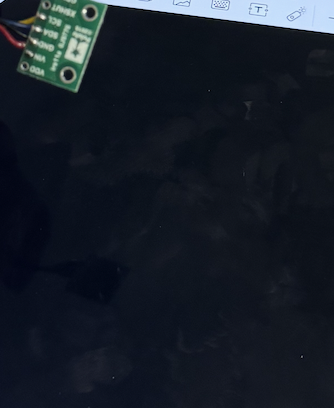
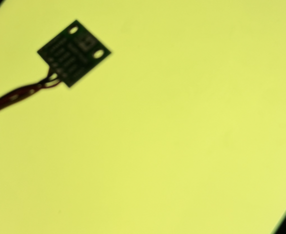
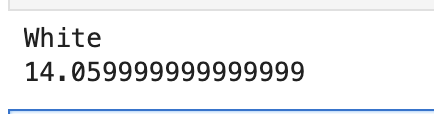
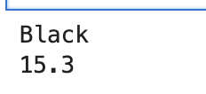
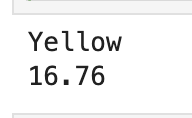
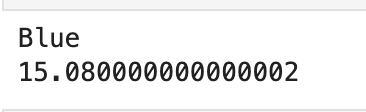
As well, I tested the ToF sensor on four different colors: white, black, yellow, and blue. All of the colors were draw on my iPad in order to keep the test consistent. Images are shown below.

As seen in the average distance output for each color below, the darker colors were more accurate than the lighter ones. This was likely a result of the increase in light emission with the lighter colors, especially since my iPad was turned on and emitting light from the screen.

###Sources: I referenced Mikayla Lahr’s website from last year when figuring out how I should wire my ToF sensors to the QWIIC connectors.